Using machine learning techniques to generate laboratory diagnostic pathways—a case study
Introduction
Laboratory diagnostic pathways combine stepwise reflex testing with economic efficacy (1). They are based on expert rules (“if…then…else”), which can be visualized as decision trees. If possible, these pathways should reflect established medical guidelines as well as local conditions, on which clinical and laboratory experts have agreed conjointly.
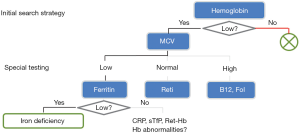
In clinical practice, diagnostic pathways represent “smart test profiles”, which are followed just to the point where a diagnostic decision can be made. A well-established example is shown in Figure 1. In contrast to traditional (inflexible) profiles, this strategy saves costs, simplifies processes, and minimizes the number of false positive and false negative results.

Machine learning algorithms may be used to either validate the decision trees established by human experts or to suggest potential new trees, if guidelines are not available. In this paper, we present and evaluate “partykit”, a statistical software tool (4), which automatically generates decision trees from real laboratory data. Although such computer-driven approaches have been pursued for quite some time (5), applications for laboratory diagnostics have been scarce so far (6-8).
In order to illustrate the algorithmic process and to discuss its benefits and limitations, we applied the decision tree learning algorithms rpart and ctree to real-life data from a published study on liver fibrosis and cirrhosis in patients with chronic hepatitis C infection (9).
Methods
From the original study group, we selected 73 patients (52 males, 21 females), aged 19 to 75 years (median 50), with a proven serological and histopathological diagnosis of hepatitis C. The morphological pictures ranged from chronic hepatitis C infection without fibrosis to end stage liver cirrhosis with a need for liver transplantation (LTX).
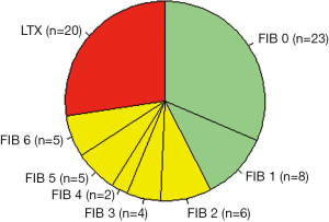
Patients were grouped into three classes (see green, yellow, and red areas in Figure 2) according to the hepatic activity index proposed by Ishak et al. (10): C1 = hepatitis without fibrosis or with only minor signs of portal fibrosis (Ishak stages F0 and F1, n=31, C2 = therapy-relevant fibrosis (Ishak stages F2 to F6, n=22), and C3 = LTX-relevant end stage liver cirrhosis [Child-Pugh stage C (11), n=20]. Liver biopsies and blood samples for the examination of biochemical measurands were taken at the same time. Figure 3 illustrates the data format.

Biochemical tests
The following six traditional diagnostic tests for liver diseases were measured on a Modular P800 automatic analyzer (Roche Diagnostics): albumin (ALB), bilirubin (BIL), choline esterase (CHE), γ-glutamyl-transferase (GGT), aspartate amino-transferase (AST), and alanine amino-transferase (ALT). The concentrations of tissue inhibitor of metalloproteinase 1 (TIMP1), N-terminal peptide of procollagen III (PIIINP), and hyaluronic acid (HA) were measured on the immunochemical analyzer ADVIA Centaur CP (Siemens). The ELF score was calculated directly by the instrument employing the following equation:
ELF score = 2.494 + 0.846 × ln(HA) + 0.735 × ln(PIIINP) + 0.391 × ln(TIMP1)
Learning decision trees
In the first part of the results section we demonstrate how decision trees can be constructed automatically from laboratory results. The algorithm selects one of the laboratory tests (attributes), splits the data set according to this test, and continues in the same way with the branches resulting from the split. This procedure stops whenever a “diagnosis” can be made, i.e., an end node (leave) is reached. Ideally, this is the case if the node contains only patients with the same diagnosis. Another stop criterion could be that the number of cases in a node becomes too small for further splitting.
In the case of the rpart algorithm, the attribute selection and splitting criterion is based on information gain (a concept derived from Shannon entropy), while the ctree algorithm uses conditional independence testing. For more details see the documentation of partykit, rpart, and ctree, which comes with the respective R packages after having installed R for Windows as described under www.r-project.org.
The following lines of code install and load the required packages:
install.packages(“partykit”)
install.packages(“rpart.plot”)
library(“partykit”)
library(“rpart.plot”)
Here is an example of a three lines code to load the dataset shown in Figure 3, and to perform the ctree algorithm:
x <- read.csv (file.choose())
t <- ctree(formula = Category~ALB+BIL+CHE+GGT+AST+ALT, data = x)
plot(t)
The first line of code loads the csv file containing the data, the second line assigns the results of the ctree function to the variable t, and the third line plots a decision tree like the one shown in Figure 4 (see results section).

The code for the rpart algorithm is very similar:
t <- rpart(formula = Category~ALB + BIL + CHE + GGT + AST + ALT, data = x)
prp(t)
Note that the generic plot function of R checks the object type of t. If it is a ctree object, it applies the type-specific plotting function plot.ctree. In the case of rpart, the specific plotting function prp must be applied.
Validation of decision trees and application to new patients
In the second part of the results section, we deal with the issue of testing and validating a decision tree learned from data. The question is how well the model will predict the diagnoses (classes) of new patients (cases).
To test the ctree mode t, we obtain the predicted class (diagnosis) for a new patient p, using the predict function of R:
predicted.class <- predict(t, p, type="class")
In the case of a decision tree generated by rpart, the type argument needs to be adapted as follows:
predicted.class <- predict(t, p, type="response")
To validate a decision tree, the classical procedure includes a training data set, on which the decision tree is constructed, and an independent test data set just for the purpose of validation. Quite often, however, the data set is too small to divide it into two data sets; this is especially true for studies like the one presented here, were the gold standard includes an invasive procedure like liver biopsy.
Therefore, we applied the leave-one-out method: validation is performed n times, where n is the total number of cases. In each cycle, one test case is removed from the data set and the rest is used as a training data set to construct a decision tree. Then the diagnosis for the patient that has been removed from the data set is predicted as described above. In this way, for each case a prediction of the corresponding diagnosis is obtained independently of the test cases. A typical algorithm for the leave-one-out method could look like this:
predicted.class <- rep(NA, n)
for (i in 1: n){
dat.training <- dat[-i,]
dat.test <- dat[i,]
t <- rpart(formula = Category~., data = dat.training)
predicted.class[i] <- predict(t, dat.test, type="class")
}
To present the results of the leave-one-out method, we used the generic table function of R to construct confusion matrices, i.e., squared contingency tables whose rows and columns correspond to the possible diagnoses, i.e., C1, C2 and C3:
table(predicted.class, dat$Category)
The rows in Table 1 indicate the predicted diagnoses P, and the columns the true diagnoses T. The entries in the diagonals are the counts of correct predictions, from which the accuracy can be calculated as a percentage of all cases.
Table 1
| Class | T1 | T2 | T3 |
|---|---|---|---|
| rpart without ELF | |||
| P1 | 21 | 14 | 2 |
| P2 | 10 | 7 | 4 |
| P3 | 0 | 1 | 14 |
| rpart with ELF | |||
| P1 | 25 | 5 | 0 |
| P2 | 3 | 14 | 4 |
| P3 | 3 | 3 | 16 |
| ctree without ELF | |||
| P1 | 28 | 10 | 2 |
| P2 | 2 | 10 | 3 |
| P3 | 1 | 2 | 15 |
| ctree with ELF | |||
| P1 | 26 | 10 | 0 |
| P2 | 5 | 8 | 5 |
| P3 | 0 | 4 | 15 |
T, true diagnoses; P, predicted diagnoses.
Accuracy was tested against random guessing using Fisher’s exact test. As a naive guess, which would not use the information from the laboratory results, we assumed that all patients fall into the predominant class 1. This guess thus yields an accuracy of 42.5% (31 correct predictions out of a total of 73 cases).
Results
Figure 5 shows boxplots for each measurand, depending on the severity of the disease (classes C1–3). The boxes comprise the central 50% of the respective test results, the thick horizontal lines represent the medians, and the circles indicate potential outliers. For better readability, the extent of the y-axes has been limited, so that a few extreme values are not displayed.

It is evident that—with the exception of GGT and transaminases—the majority of patients in class C1 have test results within the reference interval, whereas the values of the transplant candidates (class C3) are either decreased (ALB, ALT, CHE) or increased (all others). The mean values obtained in classes 1 and 2 are usually not significantly different, whereas some highly significant differences (P<0.001) are seen between classes C2 and C3 (ALB, ALT, CHE, ELF). The ELF score is the only diagnostic test, which shows significantly different mean values between all three classes. Our assumption was that the machine learning algorithms would most likely build decision trees from the diagnostic tests with the highest discriminatory power (ALB, ALT, CHE, and ELF).
Figure 6 shows two decision trees obtained with the rpart algorithm. The left tree is based on the six traditional liver tests and confirms our assumption that rpart would select ALB, ALT and CHE. Somewhat surprisingly, the algorithm adds GGT to the tree, in order to separate C2 from C1 (although the respective difference of mean values was statistically insignificant).

For the right tree in Figure 6 we added the ELF score to the input variables, and in fact we obtained a simpler picture: the rpart tree now starts with this score and predicts the existence of a grey zone between values of 9.6 and 12.0. Below this interval, class C1 is assumed, above the algorithm predicts class C3, and in between BIL is used as an additional parameter to separate C2 from C3. Interesting enough, the expected candidates ALB, ALT, and CHE are not selected.
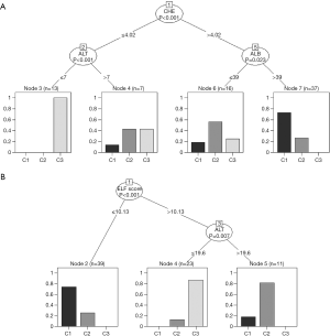
Figure 7 shows the respective results obtained with ctree. Again, the selection of ALB, ALT, and CHE in the upper part and of ELF in the lower part is in full accordance with our assumptions. Very low activities of both CHE and ALT seem to exclude classes C1 and C2.

As compared to rpart, the ctree-plots provide some additional information about how the three classes C1 to C3 are distributed within each node. A similar effect can be obtained with rpart using the following modified print command (graph not shown):
prp(t, extra=104)
Neither of the traditional tests is capable of clearly separating classes 1 and 2 from each other, whereas C3 seems to be likely, if ALT and CHE are very low (Figure 7, upper part). None of the three end nodes in the lower part of Figure 7 is composed of just one class, but the left node is clearly in favor of C1, the right one of C2, and the middle one of C3.
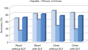
Table 1 summarizes the results of the cross-validation study based on the leave-one-out method, and Figure 4 gives an overview of the accuracies calculated from this data. It is evident that the prediction of class 1 (fibrosis with no or just slight signs of fibrosis) and class 3 (liver cirrhosis) is much better than that of class 2 (intermediate fibrosis), irrespective of the model applied. The relatively complex decision tree obtained with rpart (Figure 6, left part) seems to perform slightly worse than the other three models. Adding the ELF score to this rpart model yields the highest accuracy for class 2 (63.6%).
Taking the correct predictions for all three classes together, the rpart model with the ELF score yielded the highest accuracy (75.3%). It performed clearly better than the rpart model without ELF score and slightly better than the two ctree models. The accuracy of all four models was significantly better than that of guessing (Table 2).
Table 2
| Model | Overall accuracy (%) | P value |
|---|---|---|
| rpart without ELF | 57.5 | <0.05 |
| rpart with ELF | 75.3 | <0.001 |
| ctree without ELF | 72.6 | <0.001 |
| ctree with ELF | 67.1 | <0.01 |
It is noteworthy that the decision trees produced by multiple runs of the leave-one-out method are not necessarily identical. Any changes in the input data set may result in deviant results (for examples see Figure 8).
Discussion
Systematic reviews of the literature on chronic hepatitis C reveal that individual biochemical tests are good at separating cases with no or minimal fibrosis from those with severe fibrosis or cirrhosis; but they are poor at predicting intermediate levels of fibrosis (12). Several multivariate approaches with a potentially higher discriminatory power have been published [for a review see (13)], some of which are based on simple ratios like the AST platelet ratio index APRI (14) or on more complex equations such as the FORNS INDEX (15) and the FibroIndex (16). Stepwise approaches like the one presented in this paper are less common in the literature (17,18), and it has been only recently that machine learning was introduced as a tool for the construction of such decision trees (19).
Our study did not aim at inventing a new diagnostic algorithm for fibrosis detection, but rather at demonstrating how easy it is to automatically construct decision trees from suitable routine laboratory results. All it takes, is an installation of the free software package R (www.r-project.org) and copying a few lines of code from this publication. Illustrative graphs can be obtained without deep insight into the complex statistical methods behind the rpart and ctree functions. Even more such machine learning algorithms are included in the partykit package (4) and other programming environments (20).
Most of the decision trees presented here confirmed our initial assumption that the measurands showing significant differences between the three patient classes (see Figure 5) should be preferred by the machine learning algorithms. This was especially true for albumin and choline esterase, one of which was usually included in a root node. Whenever the ELF score, which exhibited the best discriminatory power (see Figure 5B), was included in the parameter list, this variable was selected for the root node. Interesting enough, however, some variables showing only small, insignificant differences between the three classes were also included, albeit in branches of lower order. A likely reason could be that the stepwise approach makes the subgroups more specific, so that insignificant differences become more pronounced.
Since each run of rpart or ctree took only seconds, we constructed many more trees than we could present in this article. For example, when we added the constituents of the ELF score, i.e., TIMP-1, PIIINP, and HA, to the full parameter list, ctree tended to include ELF plus TIMP-1, whereas rpart did not. In another set of experiments, we added the patients’ age to the list, since several multivariate fibrosis scores include this parameter as well. Indeed, both algorithms selected the age as a discriminator, when it was combined with the routine tests shown in Figure 5A, but not, if the ELF score was added. In fact, our patients in class 1 were significantly younger than in the other two groups (not shown).
Summarizing our observations from a medical point of view, the two most important messages are that (I) quite variable decision trees were obtained depending on the data set and the statistical method, and that (II) none of these trees was able to perfectly separate the three classes of patients (minimal, intermediate and advanced fibrosis). This may seem disappointing, but it confirms the findings in the literature [for a review see (13)], since most of the multivariate approaches published so far suffer from relatively low AUC values around 0.8 in the ROC analysis, especially when intermediate fibrosis stages are concerned.
From a statistical point of view, we would like to stress that (I) the validation of machine learning results with independent data sets is mandatory and that (II) the leave-one-out method presented here yields useful validation results if the size of the patient cohort is too small to be split into classic training and test sets. Publications, which disregard this basic requirement of independent validation, are prone to the risk of overfitting. This term means that a classifier (a ratio, index, decision tree, etc.) may work well with the original data, on which it has been developed, but will fail with data from new patients. Therefore, published accuracies are sometimes too high and exaggerate the apparent efficiency of the classifiers. To illustrate the phenomenon of overfitting, Table 3 compares the overall accuracies presented in Table 2 with those obtained without applying the leave-one-out method.
Table 3
| Model | Leave one out | Total data set |
|---|---|---|
| rpart without ELF | 57.5 | 82.2 |
| rpart with ELF | 75.3 | 83.6 |
| ctree without ELF | 72.6 | 72.6 |
| ctree with ELF | 67.1 | 79.4 |
Thus, coming back to the introductory considerations about diagnostic pathways, our machine learning approaches proved to be valuable tools, which can support but not replace the medical expert when designing decision trees. Their strength is mainly the speed, at which many alternative pathways with sometimes interesting and surprising cut-off values can be designed and tested (e.g., ALT in Figure 7). Their major weakness is that the results may look somewhat arbitrary since the algorithms do not have a clue about scientific plausibility.
Despite their popularity in medicine, simple decision trees are usually not regarded as the algorithms with the best discriminatory power. More advanced approaches such as support vector machines or deep neural networks often separate different classes better. The clear advantage of the decision trees presented here is, however, that they can easily be evaluated by medical experts, whereas the above algorithms are often black boxes.
Finally, we would like to add that a good diagnostic pathway also considers financial, organizational and eventually emotional costs of a test. Therefore tests with a high sensitivity are usually conducted early to exclude as many healthy subjects as possible from further evaluation. This behavior, which has been illustrated in Figure 1, is not replicated by automatic decision trees. An extension of decision trees that also models costs would further improve their value for the construction of diagnostic pathways. This project is currently underway.
Acknowledgments
Funding: None.
Footnote
Provenance and Peer Review: This article was commissioned by the Guest Editors (Michael Cornes and Jennifer Atherton) for the series “Reducing errors in the pre-analytical phase” published in Journal of Laboratory and Precision Medicine. The article has undergone external peer review.
Conflicts of Interest: All authors have completed the ICMJE uniform disclosure form (available at http://dx.doi.org/10.21037/jlpm.2018.06.01). The series “Reducing errors in the pre-analytical phase” was commissioned by the editorial office without any funding or sponsorship. The authors have no other conflicts of interest to declare.
Ethical Statement: The authors are accountable for all aspects of the work in ensuring that questions related to the accuracy or integrity of any part of the work are appropriately investigated and resolved.
Open Access Statement: This is an Open Access article distributed in accordance with the Creative Commons Attribution-NonCommercial-NoDerivs 4.0 International License (CC BY-NC-ND 4.0), which permits the non-commercial replication and distribution of the article with the strict proviso that no changes or edits are made and the original work is properly cited (including links to both the formal publication through the relevant DOI and the license). See: https://creativecommons.org/licenses/by-nc-nd/4.0/.
References
- Hoffmann G, Aufenanger J, Foedinger M, et al. Benefits and limitations of laboratory diagnostic pathways. Diagnosis 2014;1:269-76. [Crossref] [PubMed]
- Hofmann W, Aufenanger J, Hoffmann G, et al. editors. Laboratory diagnostic pathways. Berlin: De Gruyter, 2016.
- Thomas L, Thomas C. Detection of iron restriction in anaemic and non-anaemic patients: New diagnostic approaches. Eur J Haematol 2017;99:262-8. [Crossref] [PubMed]
- Hothorn T, Zeileis A. partykit: A modular toolkit for recursive partytioning in R. J Machine Learning Res 2015;16:3905-9.
- Murthy S. Automatic construction of decision trees from data: a multi-disciplinary survey. Data Mining and Knowledge Discovery 1998;2:345-89. [Crossref]
- Qu Y, Adam BL, Yasui Y, et al. Boosted decision tree analysis of SELDI mass spectral serum profiles discriminates prostate cancer from noncancer patients. Clin Chem 2002;48:1835-43. [PubMed]
- Dórea FC, Muckle CA, Kelton D, et al. Exploratory analysis of methods for automated classification of laboratory test orders into syndromic groups in veterinary medicine. PLoS One 2013;8:e57334 [Crossref] [PubMed]
- Metthin E, Veen J, Dekhuijzen R, et al. Development of a diagnostic decision tree for obstructive pulmonary diseases base on real-life data. ERJ Open Res 2016;2.
- Lichtinghagen R, Pietsch D, Bantel H, et al. The Enhanced Liver Fibrosis (ELF) score: Normal values, influence factors and proposed cut-off values. J Hepatol 2013;59:236-42. [Crossref] [PubMed]
- Ishak K, Baptista A, Bianchi L, et al. Histological grading and staging of chronic hepatitis. J Hepatol 1995;22:696-9. [Crossref] [PubMed]
- Pugh RN, Murray-Lyon IM, Dawson JL, et al. Transection of the oesophagus for bleeding oesophageal varices. Br J Surg 1973;60:646-9. [Crossref] [PubMed]
- Gebo KA, Herlong HF, Torbenson MS, et al. Role of liver biopsy in management of chronic hepatitis C: a systematic review. Hepatology 2002;36:S161-72. [PubMed]
- Halfon P, Bourliere M, Deydier R, et al. Independent prospective multicenter validation of biochemical markers (fibrotest-actitest) for the prediction of liver fibrosis and activity in patients with chronic hepatitis C: the fibropaca study. Am J Gastroenterol 2006;101:547-55. [Crossref] [PubMed]
- Wai CT, Greenson JK, Fontana RJ, et al. A simple noninvasive index can predict both significant fibrosis and cirrhosis in patients with chronic hepatitis C. Hepatology 2003;38:518-26. [Crossref] [PubMed]
- Forns X, Ampurdanès S, Llovet JM, et al. Identification of chronic hepatitis C patients without hepatic fibrosis by a simple predictive model. Hepatology 2002;36:986-92. [Crossref] [PubMed]
- Koda M, Matunaga Y, Kawakami M, et al. FibroIndex, a practical index for predicting significant fibrosis in patients with chronic hepatitis C. Hepatology 2007;45:297-306. [Crossref] [PubMed]
- Sebastiani G, Halton P, Castera L, et al. SAFE biopsy: a validated method for large-scale staging of liver fibrosis in chronic hepatitis C. Hepatology 2009;49:1821-7. [Crossref] [PubMed]
- Bourliere M, Penaranda G, Ouzan D, et al. Optimized stepwise combination algorithms of non-invasive liver fibrosis scores including Hepascore in hepatitis C virus patients. Aliment Pharmacol Ther 2008;28:458-67. [Crossref] [PubMed]
- Eslam M, Hashem A, Romero-Gomez M, et al. FibroGENE: a gene based model for staging liver fibrosis. J Hepatol 2016;64:390-8. [Crossref] [PubMed]
- Geurts P, Irrthum A, Wehenkel L. Supervised learning with decision tree-based methods in computational and systems biology. Mol Biosyst 2009;5:1593-605. [Crossref] [PubMed]
Cite this article as: Hoffmann G, Bietenbeck A, Lichtinghagen R, Klawonn F. Using machine learning techniques to generate laboratory diagnostic pathways—a case study. J Lab Precis Med 2018;3:58.


